Monostatic RCS measures the power of an electromagnetic wave reflected directly back to the radar source (transmitter and receiver are co-located). Mathematically, it is defined as:

$$ \sigma = \lim_{R \to \infty} 4\pi R^2 \frac{|\mathbf{E}_{\text{scattered}}|^2}{|\mathbf{E}_{\text{incident}}|^2} $$

where:

$ R $ : Distance between the radar and target.
$ \mathbf{E}_{\text{scattered}} $ : Electric field of the scattered wave.
$ \mathbf{E}_{\text{incident}} $ : Electric field of the incident wave.

In this notebook, we aim to benchmark the accuracy of Tidy3D by simulating the monostatic RCS of a PEC sphere and compare the results to the well-known analytical solution based on Mie theory.

[1]:

import tidy3d as td
import tidy3d.web as web
import numpy as np
import matplotlib.pyplot as plt

Simulation Setup¶

The monostatic RCS calculation for a PEC sphere is a classic problem in electromagnetics. The RCS is usually normalized by the physical cross section area of the sphere $\pi r^2$, where $r$ is the radius. Our goal is to calculate the normalized RCS as a function of the unitless relative frequency $2 \pi r/\lambda_0$.

In this particular case, we will calculate the RCS for a relative frequency range from 1 to 10. The result will be plotted in a log scale so the frequency points are generated in a log scale here.

[2]:

r = 1  # radius of the sphere
rel_freqs = np.logspace(0, 1, 201)  # relative frequency in log scale
ldas = 2 * np.pi * r / rel_freqs  # wavelength range
freqs = td.C_0 / ldas  # frequency range

freq0 = (freqs[-1] + freqs[0]) / 2  # central frequency for the source
fwidth = (freqs[-1] - freqs[0]) / 2  # frequency width for the source

Create the PEC sphere.

[3]:

sphere = td.Structure(geometry=td.Sphere(radius=r), medium=td.PECMedium())

Next, we define a TFSF source as the excitation. For RCS calculation, the TFSF source is the most suitable since it injects a plane wave with unit power density, which makes the normalization of the RCS calculation automatic. The source needs to enclose the sphere. The incident angle and direction do not matter due to the symmetry of the sphere but we have it injected in the $z$ axis in this case.

[4]:

source_size = 3 * r

source = td.TFSF(
    size=[source_size] * 3,
    source_time=td.GaussianPulse(freq0=freq0, fwidth=fwidth),
    injection_axis=2,
    direction="-",
)

The RCS calculation is automatically done in a FieldProjectionAngleMonitor. The monitor needs to enclose both the source and the sphere. Since we are only interested in the monostatic RCS, we only need to project to one particular angle, namely the opposite direction of the incident direction.

[5]:

monitor_size = 4 * r

monitor = td.FieldProjectionAngleMonitor(
    size=[monitor_size] * 3,
    freqs=freqs,
    name="far_field",
    phi=[0],
    theta=[0],
)

Put everything into a Simulation instance. Here we use a uniform grid of size $r$/100 to sufficiently resolve the curved surface of the sphere. By default, we apply a subpixel averaging method known as the conformal mesh scheme to PEC boundaries.

The automatic shutoff level by default is at 1e-5. Here to further push the accuracy, we lower it to 1e-8.

[6]:

run_time = 1e-13
sim_size = 6 * r

sim = td.Simulation(
    size=[sim_size] * 3,
    grid_spec=td.GridSpec.uniform(dl=r / 100),
    structures=[sphere],
    sources=[source],
    monitors=[monitor],
    run_time=run_time,
    shutoff=1e-8,
)

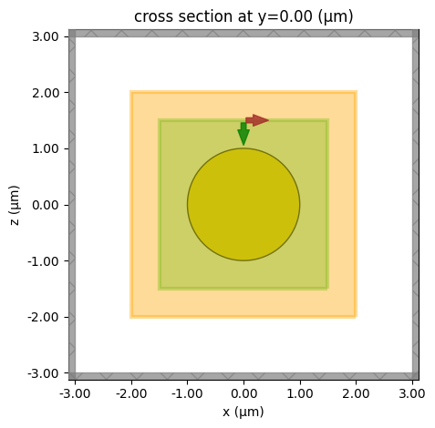
Visualize the simulation to ensure the setup is correct.

[7]:

sim.plot(y=0)
plt.show()

No description has been provided for this image

Submit the Simulation to the Server¶

Once we confirm that the simulation is set up properly, we can run it.

[8]:

sim_data = web.run(simulation=sim, task_name="pec_sphere_rcs")

16:31:40 Eastern Standard Time Created task 'pec_sphere_rcs' with task_id       
                               'fdve-2b7edb4c-ca63-448f-bfce-f531c07891eb' and  
                               task_type 'FDTD'.

                               View task using web UI at                        
                               'https://tidy3d.simulation.cloud/workbench?taskId
                               =fdve-2b7edb4c-ca63-448f-bfce-f531c07891eb'.

Output()

16:31:48 Eastern Standard Time Maximum FlexCredit cost: 0.595. Minimum cost     
                               depends on task execution details. Use           
                               'web.real_cost(task_id)' to get the billed       
                               FlexCredit cost after a simulation run.

                               status = success

Output()

16:31:49 Eastern Standard Time loading simulation from simulation_data.hdf5

Postprocessing and Visualization¶

Once the simulation is complete, we can calculate the RCS directly from the monitor data and normalize it to the physical cross section of the sphere.

[9]:

rcs_tidy3d = sim_data["far_field"].radar_cross_section.real.squeeze(drop=True).values / (
    np.pi * r**2
)

The normalized monostatic RCS (σ/πr²) of a PEC sphere is calculated using the Mie series solution:

$$ \frac{\sigma}{\pi r^2} = \frac{4}{x^2} \left| \sum_{n=1}^\infty (-1)^n (n + 0.5) \left(a_n - b_n \right) \right|^2 , $$

where:

Relative frequency:
$$ x = \frac{2\pi r}{\lambda} \quad \text{(unitless)} $$
Mie coefficients: $$ a_n = -\frac{\left[x j_n(x)\right]'}{\left[x h_n^{(1)}(x)\right]'} $$
$$ b_n = -\frac{j_n(x)}{h_n^{(1)}(x)} $$
Spherical Bessel function: $$ j_n(x) $$
Spherical Hankel function (1st kind):
$$ h_n^{(1)}(x) = j_n(x) + i y_n(x) $$

We calculate the RCS according to the formula above and compare it to the simulated RCS from Tidy3D.

[10]:

from scipy.special import spherical_jn, spherical_yn


def normalized_rcs(rel_freq):
    """
    Calculate the monostatic RCS of a PEC sphere normalized by πr².

    Parameters:
    relative_frequency (float): The relative frequency (2πr/λ), unitless.

    Returns:
    float: Normalized RCS (σ / πr²), unitless.
    """

    if rel_freq <= 0:
        return 0.0

    # determine the maximum number of terms in the series
    N_max = int(np.floor(rel_freq + 4 * rel_freq ** (1 / 3) + 2))
    total_sum = 0.0j

    for n in range(1, N_max + 1):
        # compute spherical Bessel (jn) and Neumann (yn) functions
        jn = spherical_jn(n, rel_freq)  # j_n(x)
        jn_deriv = spherical_jn(n, rel_freq, True)  # j_n'(x)

        yn = spherical_yn(n, rel_freq)  # y_n(x)
        yn_deriv = spherical_yn(n, rel_freq, True)  # y_n'(x)

        # spherical Hankel function of the first kind (hn1)
        hn1 = jn + 1j * yn  # h_n^(1)(x)
        hn1_deriv = jn_deriv + 1j * yn_deriv  # [h_n^(1)]'(x)

        # calculate (x * jn)' and (x * hn1)'
        x_jn_deriv = jn + rel_freq * jn_deriv
        x_hn1_deriv = hn1 + rel_freq * hn1_deriv

        # Mie coefficients for PEC sphere
        a_n = -x_jn_deriv / x_hn1_deriv
        b_n = -jn / hn1

        # series term
        term = ((-1) ** n) * (n + 0.5) * (a_n - b_n)
        total_sum += term

    # compute the normalized RCS
    if rel_freq == 0:
        return 0.0
    rcs_normalized = (4.0 / rel_freq**2) * (np.abs(total_sum) ** 2)
    return rcs_normalized.real


rcs_analytic = [normalized_rcs(rel_freq) for rel_freq in rel_freqs]

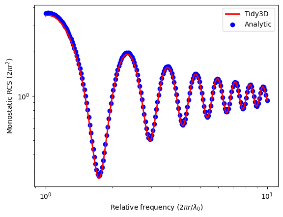
Plot the simulated and calculated RCS together. The results overlap very well, indicating the good accuracy of the Tidy3D solver.

[11]:

plt.plot(rel_freqs, rcs_tidy3d, "red", linewidth=2, label="Tidy3D")
plt.scatter(rel_freqs, rcs_analytic, c="blue", label="Analytic")
plt.xlabel("Relative frequency (2$\pi r$/$\lambda_0$)")
plt.ylabel("Monostatic RCS (2$\pi r^2$)")
plt.xscale("log")
plt.yscale("log")
plt.legend()
plt.show()

Learning Center

Monostatic radar cross section (RCS) of a PEC sphere¶

Simulation Setup¶

Submit the Simulation to the Server¶

Postprocessing and Visualization¶