A rectangular patch antenna is a type of microstrip antenna consisting of a rectangular conductive patch placed on a dielectric substrate with a ground plane on the opposite side. These antennas are widely used in wireless communication applications due to their simple design, ease of fabrication, and low profile.
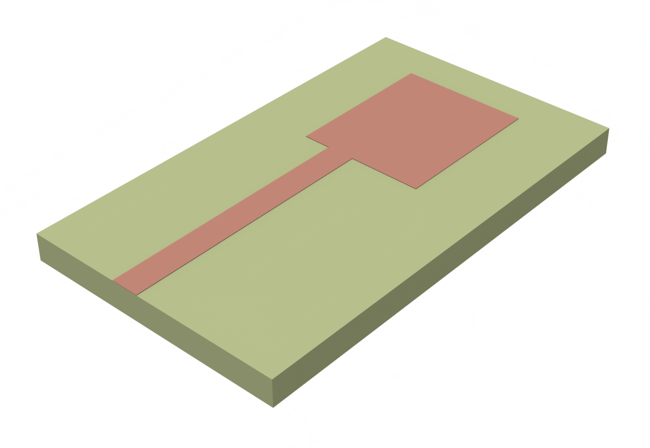
In this notebook, we will demonstrate how to use Tidy3D to simulate a rectangular patch antenna [1] and compute key performance metrics. These include S-parameters using the TerminalComponentModeler, as well as directivity, axial ratio, and polarized far-field components using the DirectivityMonitor.
# Tidy3d import
import matplotlib.pyplot as plt

# External modules needed for this notebook
import numpy as np
import tidy3d as td

# Tidy3d plugin import
import tidy3d.plugins.smatrix as smatrix
from tidy3d.web import run
Units and Frequency Settings
In Tidy3D, the default units are micrometers (µm) and Hertz (Hz). In the following, we introduce a scaling factor to convert the default unit of micrometers to millimeters (mm), which is more commonly used in antenna simulations.
# Scaling used for millimeters
mm = 1e3

# Frequency range
freq_start = 0.5e9
freq_stop = 20e9

freq0 = (freq_start + freq_stop) / 2  # Centeral frequency
freqs_target = [7.5e9, 10e9]  # Target frequencies (in Hz) for computing directivity and axial ratio
fwidth = freq_stop - freq_start  # Bandwidth

# Wavelength of centeral frequency in vacuum
wavelength0 = td.C_0 / freq0

# Frequency sweep for S-parameters
freqs = np.linspace(freq_start, freq_stop, 200)
Materials
We use a simple dielectric substrate with a relative permittivity of 2.2 and PEC2D, a thickness-free perfect electric conductor (PEC) medium to represent the conducting materials in the antenna.
# Material present
air = td.Medium()
eps_r = 2.2
sub_medium = td.Medium(permittivity=eps_r)
PEC = td.PEC2D  # Thickness-free PEC medium
Building Geometry and Structures
We follow the parameters outlined in [1] to create the corresponding patch antenna step-by-step. Boolean operations on geometries can be applied using ClipOperation.
# Substrate parameters
sub_x = 23.34 * mm
sub_y = 40 * mm
sub_z = 0.794 * mm

# Patch parameters
patch_x = 12.45 * mm
patch_y = 16 * mm

# Feedline parameters
feed_x = 2.46 * mm
feed_y = 20 * mm
feed_offset = 2.09 * mm

# Define substrate structure
substrate = td.Structure(
    geometry=td.Box(center=[0, 0, 0], size=[sub_x, sub_y, sub_z]),
    medium=sub_medium,
)

# Define ground plane structure and assign the material by PEC
ground_plane = td.Structure(
    geometry=td.Box.from_bounds(
        [-sub_x / 2, -sub_y / 2, -sub_z / 2], [sub_x / 2, sub_y / 2, -sub_z / 2]
    ),
    medium=PEC,
)

# Define patch geometry
patch_geometry = td.Box.from_bounds(
    [-patch_x / 2, -sub_y / 2 + feed_y, sub_z / 2],
    [patch_x / 2, -sub_y / 2 + feed_y + patch_y, sub_z / 2],
)

# Define feedline geometry
feedline_geometry = td.Box.from_bounds(
    [-patch_x / 2 + feed_offset, -sub_y / 2, sub_z / 2],
    [-patch_x / 2 + feed_offset + feed_x, -sub_y / 2 + feed_y, sub_z / 2],
)

# Unionize the patch and feedline
radiating_geometry = td.ClipOperation(
    operation="union", geometry_a=patch_geometry, geometry_b=feedline_geometry
)

# Define radiating structure and assign conductive patch by PEC
radiating_structure = td.Structure(
    geometry=radiating_geometry,
    medium=PEC,
)

# List of structures for the simulation.
# Arrange structures in the following order: dielectric first, followed by PEC.
# This ensures that PEC override dielectric at the interfaces.
# Reversing the order may lead to inaccurate solutions.
structures_list = [substrate, ground_plane, radiating_structure]
Define Monitors
A FieldMonitor is used to observe the field distribution on the antenna patch.
To obtain radiation characteristics such as directivity, axial ratio, and polarized far fields, use a DirectivityMonitor.
The DirectivityMonitor captures far-field information through a near-to-far field transformation.
# Field monitor to view the electromagnetic fields in the patch plane
monitor_field = td.FieldMonitor(
    center=(0, 0, sub_z / 2),
    size=(td.inf, td.inf, 0),
    freqs=freqs_target,
    name="field",
)

# Define observation parameters used for DirectitiviyMonitor
theta = np.linspace(-np.pi, np.pi, 200)
phi = np.linspace(0, np.pi, 100)

# We define a DirectivityMonitor to obtain radiation characteristics such as directivity, axial ratio and polarized far fields.
monitor_directivity = td.DirectivityMonitor(
    center=[0, 0, 0],
    size=(
        30 * mm,
        45 * mm,
        4 * mm,
    ),  # We introduce a monitor box to enclose the whole structure of interest
    freqs=freqs_target,
    name="radiation",
    phi=list(phi),
    theta=list(theta),
    far_field_approx=True,  # Far-field approximation is suitable for most cases. For more accurate far-field projections, set far_field_approx=False.
)
10:11:31 CEST WARNING: ℹ️ ⚠️ RF simulations are subject to new license
              requirements in the future. You have instantiated at least one
              RF-specific component.
Boundaries
Perfectly Matched Layers (PMLs) are applied in all directions to simulate an infinitely large domain.
# PML wavelength at 10 GHz
wl_pml = wavelength0

# Quarter wavelength (at 10 GHz) padding on each side
sim_x = sub_x + wl_pml / 2
sim_y = sub_y + wl_pml / 2
sim_z = sub_z + wl_pml / 2

# Truncate the computational domain by PMLs
boundary_spec = td.BoundarySpec(
    x=td.Boundary.pml(),
    y=td.Boundary.pml(),
    z=td.Boundary.pml(),
)
Create Simulation Object
Create a simulation object that includes all the modules we have defined. Note that the excitation (source) is not defined here and will be introduced by as a lumped port.
# Create the simulation object
sim = td.Simulation(
    center=[0, 0, 0],
    size=[sim_x, sim_y, sim_z],
    grid_spec=td.GridSpec.auto(
        min_steps_per_wvl=20,  # The largest cell size is set to 20 cells per smallest wavelength.
        wavelength=td.C_0 / freq_stop,  # Smallest wavelength to resolve
    ),
    structures=structures_list,
    sources=[],  # Sources will be added by TerminalComponentModeler
    monitors=[monitor_directivity, monitor_field],
    run_time=70 * (sub_y / td.C_0),
    boundary_spec=boundary_spec,
    plot_length_units="mm",  # This option will make plots default to units of millimeters.
)
              WARNING:  ℹ️ ⚠️ RF simulations are subject to new license
              requirements in the future. You are using RF-specific components
              in this simulation.
               - Contains monitors defined for RF wavelengths.
Define Lumped Port (Excitation) and TerminalComponentModeler
A LumpedPort is a commonly used excitation port in RF simulations. It consists of a lumped resistor at the port and a uniform current source to excite the structure.
The TerminalComponentModeler is used to combine the defined simulation object with the lumped port to compute S-parameters.
# Define the port impedance
port_impedance = 50

# Setup a LumpedPort for the TerminalComponentModeler, which is needed
# to end the port with a matched load as well as providing a source for the simulation.
port = smatrix.LumpedPort(
    center=[-patch_x / 2 + feed_offset + feed_x / 2, -sub_y / 2, 0],
    size=[feed_x, 0, sub_z],
    voltage_axis=2,
    name="lumped_port",
    impedance=port_impedance,
)

# We integrate the base simulation with the LumpedPort using the TerminalComponentModeler.
# This allows us to compute scattering parameters and extract any additional data needed from the simulation.
modeler = smatrix.TerminalComponentModeler(
    simulation=sim,
    ports=[port],
    freqs=freqs,
    verbose=True,
    remove_dc_component=False,  # Include DC component for more accuracy at low frequencies
)
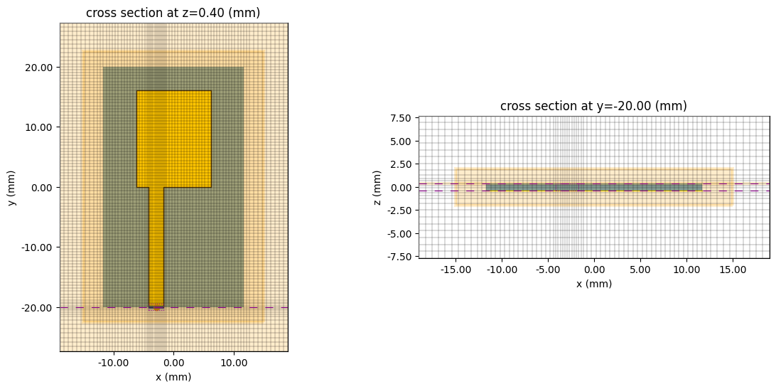
Examine Structures and Mesh
Before running the simulation, it is advisable to inspect the created structure and mesh. Here, we examine the structure along its propagation direction and the cross-section at the terminated end of the feedline, which includes the location of the lumped element.
sim_temp = list(modeler.sim_dict.values())[0]

fig, (ax1, ax2) = plt.subplots(1, 2, figsize=(14, 6))

# Examine the structure and mesh in the x-y plane
sim_temp.plot(
    z=sub_z / 2,
    ax=ax1,
    hlim=[-sim_x / 2, sim_x / 2],
    vlim=[-sim_y / 2, sim_y / 2],
    monitor_alpha=0.2,
)
sim_temp.plot_grid(z=sub_z / 2, ax=ax1, hlim=[-sim_x / 2, sim_x / 2], vlim=[-sim_y / 2, sim_y / 2])

# Examine the structure and mesh in the x-z plane
sim_temp.plot(
    y=-sub_y / 2 + 2 * mm,
    ax=ax2,
    hlim=[-sim_x / 2, sim_x / 2],
    vlim=[-sim_z / 2, sim_z / 2],
    monitor_alpha=0.2,
)
sim_temp.plot_grid(y=-sub_y / 2, ax=ax2, hlim=[-sim_x / 2, sim_x / 2], vlim=[-sim_z / 2, sim_z / 2])

# Show the plots
plt.show()
              WARNING:  ℹ️ ⚠️ RF simulations are subject to new license
              requirements in the future. You are using RF-specific components
              in this simulation.
               - Contains a 'LumpedElement'.
               - Contains monitors defined for RF wavelengths.
              WARNING: Structure at structures[0] was detected as being less
              than half of a central wavelength from a PML on side x-min. To
              avoid inaccurate results or divergence, please increase gap
              between any structures and PML or fully extend structure through
              the pml.
WARNING: Suppressed 17 WARNING messages.
Run simulation
td.config.logging_level = "ERROR"

batch_data = {
    task_name: run(simulation=simulation, task_name="AntennaCharacteristics")
    for task_name, simulation in modeler.sim_dict.items()
}
10:11:33 CEST Created task 'AntennaCharacteristics' with task_id
              'fdve-5060434e-f2b3-4287-bfa6-f08bc5cbf4df' and task_type 'FDTD'.
              View task using web UI at
              'https://tidy3d.simulation.cloud/workbench?taskId=fdve-5060434e-f2
              b3-4287-bfa6-f08bc5cbf4df'.
Task folder: 'default'.
Output()
10:11:35 CEST Maximum FlexCredit cost: 0.025. Minimum cost depends on task
              execution details. Use 'web.real_cost(task_id)' to get the billed
              FlexCredit cost after a simulation run.
10:11:36 CEST status = success
Output()
10:11:39 CEST loading simulation from simulation_data.hdf5
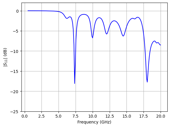
Post processing: S-parameters
s_matrix = modeler._construct_smatrix()

plt.plot(
    s_matrix.f / 1e9,
    20 * np.log10(np.abs(s_matrix.isel(port_out=0, port_in=0).values.flatten())),
    "-b",
)

plt.xlabel("Frequency (GHz)")
plt.ylabel("$|S_{11}|$ (dB)")
plt.ylim(-25, 2)
plt.grid(True)
plt.show()
Output()
10:11:42 CEST Started working on Batch containing 1 tasks.
10:11:44 CEST Maximum FlexCredit cost: 0.025 for the whole batch.
              Use 'Batch.real_cost()' to get the billed FlexCredit cost after
              the Batch has completed.
Output()
Batch complete.
Output()
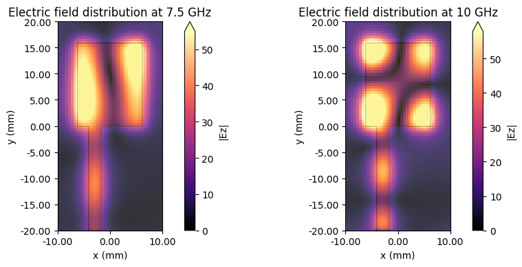
Post processing: Field distributions
sim_data = batch_data["smatrix_lumped_port"]

f, (ax1, ax2) = plt.subplots(1, 2, tight_layout=True, figsize=(11, 4))
sim_data.plot_field(
    field_monitor_name="field", field_name="Ez", val="abs", f=freqs_target[0], ax=ax1
)
ax1.set_xlim([-10 * mm, 10 * mm])
ax1.set_ylim([-20 * mm, 20 * mm])
ax1.set_title("Electric field distribution at 7.5 GHz")

sim_data.plot_field(
    field_monitor_name="field", field_name="Ez", val="abs", f=freqs_target[1], ax=ax2
)
ax2.set_xlim([-10 * mm, 10 * mm])
ax2.set_ylim([-20 * mm, 20 * mm])
ax2.set_title("Electric field distribution at 10 GHz");
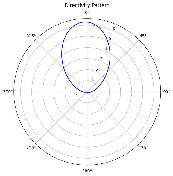
Post processing: Directivity
Directivity is a dimensionless quantity defined as the ratio of the radiation intensity in a given direction to the average radiation intensity over all directions. Mathematically, directivity $D(\theta, \phi)$ in a given direction $(\theta, \phi)$ is defined as:
$$ D(\theta, \phi) = \frac{4\pi}U(\theta, \phi)}{P_{\text{rad}} $$
where:
- $U(\theta, \phi)$: Radiation intensity in direction $(\theta, \phi)$
- $P_{\text{rad}}$: Total radiated power
Computation
-
Radiation Intensity:
Radiation intensity is given by:$$ U(\theta, \phi) = r^2 \cdot S_{\text{rad}}(\theta, \phi) $$
where $S_{\text{rad}}(\theta, \phi)$ is the far-field Poynting vector magnitude, computed as:
$$ S_{\text{rad}}(\theta, \phi) = \frac{1}{2} \cdot \text{Re}(E_\theta H_\phi^* - E_\phi H_\theta^*) $$
Here, $E_\theta$ and $E_\phi$ are the electric field components in the far-field, $H_\phi^*$ and $H_\theta^*$ are the complex conjugates of the magnetic field components, and $r$ is the distance from the source.
-
Total Radiated Power:
The total radiated power is computed by integrating the Poynting vector over the sphere:$$ P_{\text{rad}} = \int_{0}^{2\pi} \int_{0}^{\pi} S_{\text{rad}}(\theta, \phi) r^2 \sin\theta \, d\theta \, d\phi $$
-
Directivity:
Directivity is determined by substituting $U(\theta, \phi)$ and $P_{\text{rad}}$ into the formula:$$ D(\theta, \phi) = \frac{4\pi}U(\theta, \phi)}{P_{\text{rad}} $$
def log_value(values):
    return 20 * np.log10(values)


# Extract directivity
D_directivity = sim_data["radiation"].directivity.sel(f=freqs_target[0], phi=0, method="nearest")
D_directivity = np.squeeze(D_directivity)

# Create a single polar plot
fig = plt.figure(figsize=(8, 6), tight_layout=True)
ax = fig.add_subplot(111, projection="polar")

# Plot directivity
ax.set_theta_direction(-1)
ax.set_theta_offset(np.pi / 2.0)
ax.plot(theta, D_directivity, "-b", label="Tidy3D")
ax.set_title("Directivity Pattern", va="bottom")

plt.show()
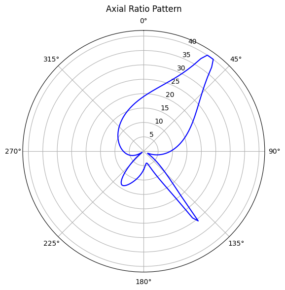
Post processing: Axial Ratio
AR is a dimensionless quantity defined as the ratio of the major axis to the minor axis of the polarization ellipse $$ AR = \frac{E_{\text{major}}}{E_{\text{minor}}} $$
For a perfectly circularly polarized wave, $ AR = 1 $, corresponding to 0 dB.
Computation:
The complex far field components $E_\theta$ and $E_\phi$ are used to determine the AR:
$$AR = \sqrt{\frac{|E_\theta|^2 + |E_\phi|^2 + |E_\theta^2 + E_\phi^2|}{|E_\theta|^2 + |E_\phi|^2 - |E_\theta ^2 + E_\phi^2|}}$$
# Extract axial ratio
AxialRatio = sim_data["radiation"].axial_ratio.sel(f=freqs_target[0], phi=0, method="nearest")
AxialRatio = np.squeeze(AxialRatio)

# Create a single polar plot
fig = plt.figure(figsize=(8, 6), tight_layout=True)
ax = fig.add_subplot(111, projection="polar")

# Plot axial ratio
ax.set_theta_direction(-1)
ax.set_theta_offset(np.pi / 2.0)
ax.plot(theta, log_value(AxialRatio), "-b", label="Tidy3D")
ax.set_title("Axial Ratio Pattern", va="bottom")

plt.show()
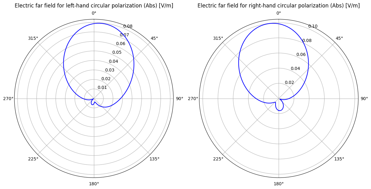
Post processing: Left and Right polarized far field
Left polarization represents the counter-clockwise component of circularly polarized electric fields, calculated as:
$$ E_{\text{left}} = \frac{E_\theta - j E_\phi}{\sqrt{2}} $$
while right polarization represents the clockwise component, calculated as:
$$ E_{\text{right}} = \frac{E_\theta + j E_\phi}{\sqrt{2}} $$
# Extract left polarization
left_polarization = abs(
    sim_data["radiation"].left_polarization.sel(f=freqs_target[0], phi=0, method="nearest")
)
left_polarization = np.squeeze(left_polarization)

# Extract right polarization
right_polarization = abs(
    sim_data["radiation"].right_polarization.sel(f=freqs_target[0], phi=0, method="nearest")
)
right_polarization = np.squeeze(right_polarization)

fig, (ax1, ax2) = plt.subplots(
    1, 2, subplot_kw={"projection": "polar"}, figsize=(12, 6), tight_layout=True
)

# Plot left polarization
ax1.set_theta_direction(-1)
ax1.set_theta_offset(np.pi / 2.0)
ax1.plot(theta, abs(left_polarization), "-b", label="Tidy3D")
ax1.set_title("Electric far field for left-hand circular polarization (Abs) [V/m]", va="bottom")

# Plot right polarization
ax2.set_theta_direction(-1)
ax2.set_theta_offset(np.pi / 2.0)
ax2.plot(theta, abs(right_polarization), "-b", label="Tidy3D")
ax2.set_title("Electric far field for right-hand circular polarization (Abs) [V/m]", va="bottom")

plt.show()
Reference
[1] Sheen, D.M., Ali, S.M., Abouzahra, M.D. and Kong, J.A., 1990. Application of the three-dimensional finite-difference time-domain method to the analysis of planar microstrip circuits. IEEE Transactions on microwave theory and techniques, 38(7), pp.849-857.