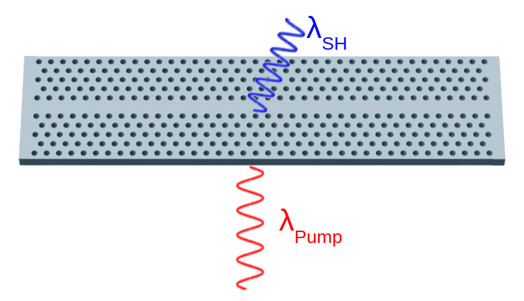
This notebook demonstrates how to use linear fields to calculate the nonlinear polarization and apply it as a source to investigate Second Harmonic Generation (SHG) in a 2D photonic crystal cavity reported in the work of Heungjoon Kim, Bong-Shik Song, Takashi Asano and Susumu Noda, entitled "Enhanced second-harmonic generation in a photonic crystal waveguide-coupled nanocavity using a wavelength-selective reflector", APL Photonics, 2023. DOI: https://doi.org/10.1063/5.0173196

We will achieve this in two steps:

Run a linear simulation with a GaussianPulse source to determine the resonant frequency and resonant fields.
Run a CW simulation exciting the resonance frequency until reach the steady state.
Use the linear field information to create the nonlinear polarization,

$$P^{(2)}_{i,j,k} = \epsilon_0 d_{i,j,k} E_j E_k$$

transform to current with the relation,

$$P^{(2)}(\vec{r},t) = \frac{\partial J^{(2)}}{\partial t} == -i \omega_{sh} P^{(2)}(\vec{r})$$

and apply it as CustomCurrentSource.

In this notebook, we will explore various features of Tidy3D, such as:

Anisotropic media.
Using ResonanceFinder to extract resonance information from time-domain field monitors efficiently.
Using a CustomCurrentSource.

This notebook example was kindly shared by the Brightlight Photonics team.

[1]:

# Standard python imports
import numpy as np
import matplotlib.pyplot as plt

import tidy3d as td

from tidy3d import web
from tidy3d.plugins.resonance import ResonanceFinder

import jupyter_black

jupyter_black.load()

Parameters Definition¶

Here, we define the global parameters for the simulation as well as the anisotropic medium.

[2]:

# Universal parameters

ep_hole = 1  # Dielectric constant of the holes

n_ordinary_1550nm = 2.564
n_extraordinary_1550nm = 2.608

n_ordinary_775nm = 2.607
n_extraordinary_775nm = 2.65

# Defining anisotropic materials
medium_xx_1550 = td.Medium(permittivity=n_ordinary_1550nm**2)
medium_yy_1550 = td.Medium(permittivity=n_ordinary_1550nm**2)
medium_zz_1550 = td.Medium(permittivity=n_extraordinary_1550nm**2)

mat_slab_1550 = td.AnisotropicMedium(
    xx=medium_xx_1550, yy=medium_yy_1550, zz=medium_zz_1550, name="mat_slab"
)
mat_hole_1550 = td.Medium(permittivity=ep_hole, name="mat_hole")

medium_xx_775 = td.Medium(permittivity=n_ordinary_775nm**2)
medium_yy_775 = td.Medium(permittivity=n_ordinary_775nm**2)
medium_zz_775 = td.Medium(permittivity=n_extraordinary_775nm**2)

mat_slab_775 = td.AnisotropicMedium(
    xx=medium_xx_775, yy=medium_yy_775, zz=medium_zz_775, name="mat_slab"
)
mat_hole_775 = td.Medium(permittivity=ep_hole, name="mat_hole")

a_lattice = 0.530
r_hole = 0.26
t_slab = 0.57
sidewall_angle = 0
sim_size = Lx, Ly, Lz = (a_lattice * 40, a_lattice * np.sqrt(3) / 2 * 12, 3)

Now we define the photonic crystal cavity geometry.

[3]:

# potential well on half-integer grid
def sqrt_potential(depth, width, n_max=100, plot=False):
    x_points = np.arange(0, n_max, 0.5)
    potential = np.sqrt(np.interp(x_points, [0, width, n_max], [depth, 0, 0]))
    if plot:
        plt.scatter(x_points, potential)

    return x_points, potential


# potential well on half-integer grid
def linear_potential(depth, width, n_max=100, plot=False):
    x_points = np.arange(0, n_max, 0.5)
    potential = np.interp(x_points, [0, width, n_max], [depth, 0, 0])
    if plot:
        plt.scatter(x_points, potential)

    return x_points, potential


def noda_potential(n_max=100):
    x_points = np.arange(0, n_max, 0.5)
    potential = np.interp(
        x_points,
        [0, 0.5, 1.5, 2, 2.5, 3, 3.5, n_max],
        [0.0094, 0.0094, 0.0047, 0.0047, 0.0047, 0, 0, 0],
    )
    return x_points, potential


def normed_x_hole_position_from_potential(x, y):
    cumsum = np.cumsum(y + 1) * 0.5
    return x, cumsum - cumsum[0]


def define_geometry(mat_slab, mat_hole):
    vector_1_normed = np.array([1 / 2, np.sqrt(3) / 2])
    vector_2_normed = np.array([-1 / 2, np.sqrt(3) / 2])

    period_indices, x_position_normed = normed_x_hole_position_from_potential(*noda_potential())

    num_periods = 80
    sim_lim_x = Lx / 2 - a_lattice / 2
    sim_lim_y = Ly / 2 - a_lattice / 2

    hole_positions = []
    for a1 in np.arange(-num_periods, num_periods):
        for a2 in np.arange(-num_periods, num_periods):
            normed_lattice_coord = a1 * vector_1_normed + a2 * vector_2_normed

            x_lattice_index = normed_lattice_coord[0]

            if x_lattice_index < 0:
                continue

            matches = np.where(period_indices == x_lattice_index)[0]
            if len(matches) != 1:
                print(x_lattice_index)
                continue

            final_hole_coord = a_lattice * np.array(
                [x_position_normed[matches[0]], normed_lattice_coord[1]]
            )

            if sim_lim_y >= final_hole_coord[1] > 0 and 0 <= final_hole_coord[0] < sim_lim_x:
                hole_positions.append(final_hole_coord)

    # reflect along y:
    hole_positions_reflected_x = []

    for pos in hole_positions:
        if pos[0] > a_lattice / 10:
            hole_positions_reflected_x.append([-pos[0], pos[1]])

    hole_positions.extend(hole_positions_reflected_x)

    hole_positions.extend([[pos[0], -pos[1]] for pos in hole_positions])

    hole_positions = np.array(hole_positions)

    plot = False
    if plot:
        plt.scatter(hole_positions[:, 0], hole_positions[:, 1])
        plt.axis("equal")
        # plt.xlim(0, 1)
        plt.show()

    slab = td.Structure(
        geometry=td.Box(
            center=(0, 0, 0),
            size=(td.inf, td.inf, t_slab * a_lattice),
        ),
        medium=mat_slab,
        name="slab",
    )

    holes = []
    for hole_pos in hole_positions:
        holes.append(
            td.Structure(
                geometry=td.Cylinder(
                    center=(hole_pos[0], hole_pos[1], 0),
                    axis=2,
                    radius=r_hole * a_lattice,
                    length=t_slab * a_lattice,
                    sidewall_angle=-sidewall_angle * np.pi / 180,
                ),
                medium=mat_hole,
                name="hole_" + str(len(holes)),
            )
        )

    structures = [slab] + holes
    return structures

[4]:

structures_list = define_geometry(mat_slab_1550, mat_hole_1550)

Gaussian Pulse Simulation¶

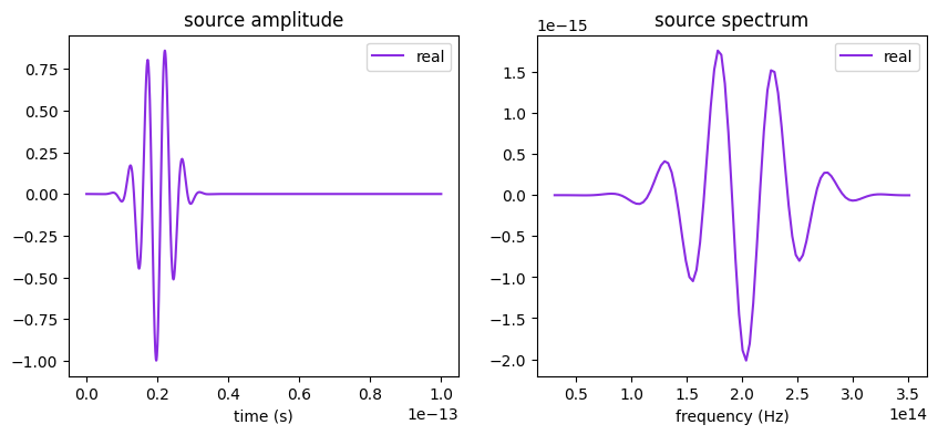
First, we define a PointDipole source with Gaussian time dependency.

[5]:

# Central frequency around which we'll look for the cavity mode (Hz)
freq0 = 1.908e14

# Source bandwidth (Hz)
fwidth = 4e13

# Simulation run time (s)
run_time = 20e-12

# Plot time dependence to verify when the source pulse decayed
source = td.PointDipole(
    center=(0, 0, 0),
    source_time=td.GaussianPulse(freq0=freq0, fwidth=fwidth),
    polarization="Ey",
)

# Source pulse is much shorter than the simulation run_time defined above,
# so we only examine the signal up to a shorter time = 10e-13fs
fig, ax = plt.subplots(1, 2, figsize=(10, 4))
source.source_time.plot(np.linspace(0, 1e-13, 2000), ax=ax[0])
source.source_time.plot_spectrum(times=np.linspace(0, 5e-13, 2000), ax=ax[1])
plt.show()

No description has been provided for this image

[6]:

# Suppress warnings for some of the holes being too close to the PML
td.config.logging_level = "ERROR"

refine_box = td.MeshOverrideStructure(
    geometry=td.Box(center=(0, 0, 0), size=(td.inf, td.inf, t_slab * a_lattice)),
    dl=[None, None, t_slab * a_lattice / 12],
)

# Mesh step in x, y, z, in microns
steps_per_unit_length_xy = 15
steps_per_unit_length_z = 15
grid_spec = td.GridSpec(
    grid_x=td.AutoGrid(min_steps_per_wvl=steps_per_unit_length_xy),
    grid_y=td.AutoGrid(min_steps_per_wvl=steps_per_unit_length_xy),
    grid_z=td.AutoGrid(min_steps_per_wvl=steps_per_unit_length_z),
    override_structures=[refine_box],
)

# Starting time after the source has decayed
t_start = 10e-13

# Time series monitor for Q-factor computation
time_series_mnt = td.FieldTimeMonitor(
    center=[0, 0, 0], size=[0, 0, 0], start=t_start, name="time_series"
)

# Flux time  monitor
flux_time = td.FluxTimeMonitor(
    center=(0, 0, 0), size=(0.8 * Lx, 0.8 * Ly, 0.8 * Lz), name="flux_time"
)

eps_monitor = td.PermittivityMonitor(
    center=(0, 0, 0), size=(Lx, Ly, Lz), freqs=[freq0], name="eps_monitor"
)

apodization = td.ApodizationSpec(start=t_start, width=2e-13)
field_mnt = td.FieldMonitor(
    center=(0, 0, 0),
    size=(Lx, Ly, Lz),
    name="field_mnt",
    freqs=[freq0],
    apodization=apodization,
)


sim = td.Simulation(
    size=sim_size,
    grid_spec=grid_spec,
    structures=structures_list,
    sources=[source],
    monitors=[time_series_mnt, flux_time, field_mnt, eps_monitor],
    run_time=run_time,
    boundary_spec=td.BoundarySpec(x=td.Boundary.pml(), y=td.Boundary.pml(), z=td.Boundary.pml()),
    symmetry=(1, -1, 1),
)

[7]:

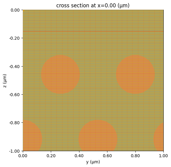
# Plot simulation and overlay grid in the xy planes
def plot_sim_grid(sim):
    fig, ax = plt.subplots(1, 1, figsize=(12, 6))
    sim.plot(z=0, ax=ax, monitor_alpha=0)
    sim.plot_grid(x=0, ax=ax, lw=0.4, colors="r")
    plt.ylim(-1, 0)
    plt.xlim(0, 1)
    print(f"Total number of grid points (millions): {sim.num_cells / 1e6:1.2}")

    return ax


plot_sim_grid(sim)
plt.show()

Total number of grid points (millions): 6.6

[8]:

# Visualize simulation
sim.plot_3d()

[9]:

# Running the simulation
sim_data = web.run(sim, task_name="1_fundamental_mode_spectrum")

20:59:33 -03 Created task '1_fundamental_mode_spectrum' with task_id            
             'fdve-1ac35438-20c7-465f-8690-ce810e8c5bd7' and task_type 'FDTD'.

             View task using web UI at                                          
             'https://tidy3d.simulation.cloud/workbench?taskId=fdve-1ac35438-20c
             7-465f-8690-ce810e8c5bd7'.

             Task folder: 'default'.

Output()

20:59:36 -03 Maximum FlexCredit cost: 0.194. Minimum cost depends on task       
             execution details. Use 'web.real_cost(task_id)' to get the billed  
             FlexCredit cost after a simulation run.

20:59:38 -03 status = queued

             To cancel the simulation, use 'web.abort(task_id)' or              
             'web.delete(task_id)' or abort/delete the task in the web UI.      
             Terminating the Python script will not stop the job running on the 
             cloud.

Output()

20:59:43 -03 status = preprocess

20:59:47 -03 starting up solver

20:59:48 -03 running solver

Output()

21:01:51 -03 status = postprocess

Output()

21:01:55 -03 status = success

21:01:57 -03 View simulation result at                                          
             'https://tidy3d.simulation.cloud/workbench?taskId=fdve-1ac35438-20c
             7-465f-8690-ce810e8c5bd7'.

Output()

21:02:10 -03 loading simulation from simulation_data.hdf5

[10]:

eps_non_colocated = abs(sim_data["eps_monitor"].eps_yy).isel(f=0)

eps = eps_non_colocated.interp(
    x=sim_data["field_mnt"].Ex.coords["x"],
    y=sim_data["field_mnt"].Ex.coords["y"],
    z=sim_data["field_mnt"].Ex.coords["z"],
)

[11]:

ax = sim_data.plot_field(
    "field_mnt",
    "Ey",
    "real",
    z=0,
    robust=False,
    eps_alpha=0,
)

ax.pcolormesh(eps.x, eps.y, eps.sel(z=0, method="nearest").real.T, alpha=0.2, cmap="binary")


plt.show()

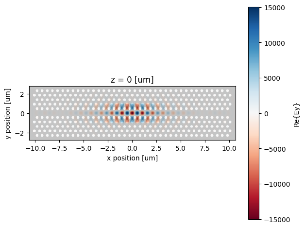
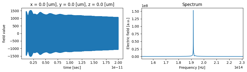
Now, we will analyze the field time series data. As we can see, the resonances exhibit exponential decay, and the cavity resonance is clearly visible in the Fourier transform.

[12]:

# Get data from the TimeMonitor
tdata = sim_data["time_series"]

time_series = tdata.Ey.squeeze()


fig, (ax1, ax2) = plt.subplots(1, 2, figsize=(10, 3))

# Plot time dependence
time_series.plot(ax=ax1)

# Make frequency mesh and plot spectrum
dt = sim_data.simulation.dt

fmesh = np.linspace(-1 / dt / 2, 1 / dt / 2, time_series.size)
spectrum = np.fft.fftshift(np.fft.fft(time_series))

ax2.plot(fmesh, np.abs(spectrum))
ax2.set_xlim(freq0 - fwidth, freq0 + fwidth)
ax2.set_xlabel("Frequency [Hz]")
ax2.set_ylabel("Electric field [a.u.]")
ax2.set_title("Spectrum")

plt.tight_layout()

plt.show()

Now we can use ResonanceFinder to calculate the resonant frequency and Q-factor:

[13]:

resonance_finder = ResonanceFinder(
    freq_window=(freq0 - fwidth / 2, freq0 + fwidth / 2), init_num_freqs=100
)
resonance_data = resonance_finder.run(sim_data["time_series"])
resonance_data.to_dataframe()

[13]:

	decay	Q	amplitude	phase	error
freq
1.916514e+14	1.265659e+10	47571.325619	676.657889	0.715587	0.000618
1.921427e+14	2.446458e+11	2467.380475	76.432467	-2.481902	0.000839
1.926705e+14	7.228575e+11	837.360110	82.764169	0.594612	0.002911
1.934497e+14	1.414883e+12	429.533819	46.411220	2.004166	0.021042

[14]:

cavity_resonance_freq = float(resonance_data.freq[0])

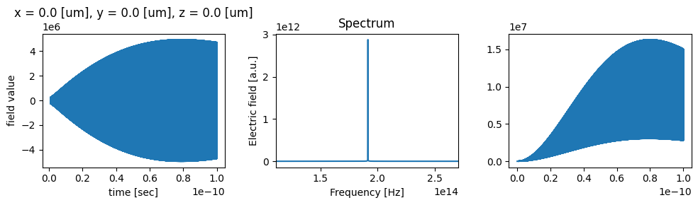
CW Run¶

Now, we will run a CW simulation at the resonance frequency until the fields reach a steady state. Then, we will record the fields and use them in the calculation of the nonlinear polarization.

[15]:

run_time_cw = 1e-10
field_mnt_time = td.FieldTimeMonitor(
    center=(0, 0, 0),
    size=(Lx, Ly, Lz),
    fields=["Ex", "Ey", "Ez"],
    start=run_time_cw - 1 / freq0,
    interval=1,
    colocate=True,
    name="movie_monitor",
)

sim_cw = sim.updated_copy(
    sources=(
        td.PointDipole(
            center=(0, 0, 0),
            source_time=td.ContinuousWave(freq0=cavity_resonance_freq, fwidth=fwidth),
            polarization="Ey",
        ),
    ),
    monitors=list(sim.monitors) + [field_mnt_time],
    run_time=run_time_cw,
)

sim_data_cw = web.run(sim_cw, task_name="1_fundamental_mode_spectrumCW")

21:02:14 -03 Created task '1_fundamental_mode_spectrumCW' with task_id          
             'fdve-8db353fb-06d6-4282-81e2-8f02a9c287c2' and task_type 'FDTD'.

             View task using web UI at                                          
             'https://tidy3d.simulation.cloud/workbench?taskId=fdve-8db353fb-06d
             6-4282-81e2-8f02a9c287c2'.

             Task folder: 'default'.

Output()

21:02:17 -03 Maximum FlexCredit cost: 0.995. Minimum cost depends on task       
             execution details. Use 'web.real_cost(task_id)' to get the billed  
             FlexCredit cost after a simulation run.

21:02:19 -03 status = queued

             To cancel the simulation, use 'web.abort(task_id)' or              
             'web.delete(task_id)' or abort/delete the task in the web UI.      
             Terminating the Python script will not stop the job running on the 
             cloud.

Output()

21:02:26 -03 status = preprocess

21:02:31 -03 starting up solver

             running solver

Output()

21:12:16 -03 status = postprocess

Output()

21:13:03 -03 status = success

21:13:05 -03 View simulation result at                                          
             'https://tidy3d.simulation.cloud/workbench?taskId=fdve-8db353fb-06d
             6-4282-81e2-8f02a9c287c2'.

Output()

21:14:40 -03 loading simulation from simulation_data.hdf5

[16]:

# Get data from the TimeMonitor
tdata = sim_data_cw["time_series"]

time_series = tdata.Ey.squeeze()

# Get data from the TimeMonitor
tdata_flux = sim_data_cw["flux_time"]

flux = tdata_flux.flux.squeeze()
time_flux = tdata_flux.flux.coords["t"]

fig, (ax1, ax2, ax3) = plt.subplots(1, 3, figsize=(10, 3))

# Plot time dependence
time_series.plot(ax=ax1)

# Make frequency mesh and plot spectrum
dt = sim_data_cw.simulation.dt
fmesh = np.linspace(-1 / dt / 2, 1 / dt / 2, time_series.size)
spectrum = np.fft.fftshift(np.fft.fft(time_series))

ax2.plot(fmesh, np.abs(spectrum))
ax2.set_xlim(freq0 - 2 * fwidth, freq0 + 2 * fwidth)
ax2.set_xlabel("Frequency [Hz]")
ax2.set_ylabel("Electric field [a.u.]")
ax2.set_title("Spectrum")

ax3.plot(time_flux, np.abs(flux))

plt.tight_layout()

plt.show()

[17]:

max_field_coord = sim_data_cw["movie_monitor"].Ey.idxmax(dim="t")

Ey_array = np.array(sim_data_cw["movie_monitor"].Ey)
integrated_ey_time = np.sum(Ey_array, axis=(0, 1, 2))
time_coord_max_field = np.argmax(integrated_ey_time)

[18]:

Ex = sim_data_cw["movie_monitor"].Ex.isel(t=time_coord_max_field).drop("t")
Ey = sim_data_cw["movie_monitor"].Ey.isel(t=time_coord_max_field).drop("t")
Ez = sim_data_cw["movie_monitor"].Ez.isel(t=time_coord_max_field).drop("t")

/tmp/ipykernel_28045/4225370433.py:1: DeprecationWarning: dropping variables using `drop` is deprecated; use drop_vars.
  Ex = sim_data_cw["movie_monitor"].Ex.isel(t=time_coord_max_field).drop("t")
/tmp/ipykernel_28045/4225370433.py:2: DeprecationWarning: dropping variables using `drop` is deprecated; use drop_vars.
  Ey = sim_data_cw["movie_monitor"].Ey.isel(t=time_coord_max_field).drop("t")
/tmp/ipykernel_28045/4225370433.py:3: DeprecationWarning: dropping variables using `drop` is deprecated; use drop_vars.
  Ez = sim_data_cw["movie_monitor"].Ez.isel(t=time_coord_max_field).drop("t")

The SHG will only occur in the nonlinear medium, so we will create a mask to exclude the holes.

[19]:

# Permittivity distribution.
eps_non_colocated = abs(sim_data_cw["eps_monitor"].eps_yy).isel(f=0)

eps = eps_non_colocated.interp(
    x=Ex.coords["x"],
    y=Ex.coords["y"],
    z=Ex.coords["z"],
)


eps_max = np.max(np.real(eps))

nonlinear_material_mask = np.real(eps) - 1
nonlinear_material_mask = nonlinear_material_mask / np.max(nonlinear_material_mask)

[20]:

tdata_flux_w0 = sim_data_cw["flux_time"]
flux_w0 = tdata_flux_w0.flux.squeeze()
radiated_power = float(np.mean(flux_w0[int(len(flux_w0) * 0.99) : -1]))

[21]:

# Compute energy in cavity
integrand = eps * (Ex * np.conjugate(Ex) + Ey * np.conjugate(Ey) + Ez * np.conjugate(Ez))
integrated_energy = td.EPSILON_0 / 2 * integrand.integrate(coord=("x", "y", "z")).item()
Q = (integrated_energy / radiated_power) * 2 * np.pi * cavity_resonance_freq

print(Q)

47623.6432485041

Second Harmonic Simulation¶

Defining the relevant polarization tensor

[22]:

# Calculating the second-order nonlinear polarization
d15 = 6.7 * 1e-6  # um/V
d31 = 6.5 * 1e-6  # um/V
d33 = -11.7 * 1e-6  # um/V

# Central frequency around which we'll look for the cavity mode (Hz)
freq_SH = 2 * cavity_resonance_freq

Now, we will define the relevant polarization fields using the relation: $P_{i,j,k} = \omega_0 \epsilon_0 d_{i,j,k} E_j E_k$.

[23]:

Pxxz = td.EPSILON_0 * d15 * nonlinear_material_mask * Ex * Ez
Pyyz = td.EPSILON_0 * d15 * nonlinear_material_mask * Ey * Ez
Pzxx = td.EPSILON_0 * d31 * nonlinear_material_mask * Ex * Ex
Pzyy = td.EPSILON_0 * d31 * nonlinear_material_mask * Ey * Ey
Pzzz = td.EPSILON_0 * d33 * nonlinear_material_mask * Ez * Ez


Pxxz = Pxxz.expand_dims(dim={"f": 1}, axis=3)
Pyyz = Pyyz.expand_dims(dim={"f": 1}, axis=3)
Pzxx = Pzxx.expand_dims(dim={"f": 1}, axis=3)
Pzyy = Pzyy.expand_dims(dim={"f": 1}, axis=3)
Pzzz = Pzzz.expand_dims(dim={"f": 1}, axis=3)

Pxxz = Pxxz.assign_coords(f=[freq_SH])
Pyyz = Pyyz.assign_coords(f=[freq_SH])
Pzxx = Pzxx.assign_coords(f=[freq_SH])
Pzyy = Pzyy.assign_coords(f=[freq_SH])
Pzzz = Pzzz.assign_coords(f=[freq_SH])

Finally, we create the polarization dataset to be used in the CustomCurrentSource

[24]:

factor = -1j * (freq_SH * 2 * np.pi)
polarization = td.FieldDataset(
    Ex=factor * Pxxz,
    Ey=factor * Pyyz,
    Ez=factor * (Pzxx + Pzyy + Pzzz),
)

[25]:

# Source bandwidth (Hz)
fwidth_SH = freq_SH * 0.3

# Simulation run time (s)
run_time_SH = 2e-12

# In-built GaussianBeam source
pulse = td.ContinuousWave(freq0=freq_SH, fwidth=fwidth_SH)

custom_src_JM = td.CustomCurrentSource(
    source_time=pulse,
    center=(0, 0, 0),
    size=(Lx, Ly, Lz),
    current_dataset=polarization,
)

[26]:

structures_775 = define_geometry(mat_slab_775, mat_hole_775)

simSH = td.Simulation(
    size=sim.size,
    grid_spec=td.GridSpec.from_grid(
        sim.grid
    ),  # Reference to the linear simulation for copying the grid
    structures=structures_775,
    sources=[custom_src_JM],
    monitors=[time_series_mnt, eps_monitor, flux_time, field_mnt],
    run_time=run_time_SH,
    boundary_spec=td.BoundarySpec(x=td.Boundary.pml(), y=td.Boundary.pml(), z=td.Boundary.pml()),
    symmetry=(0, 0, 0),
    shutoff=0,
)

[27]:

sim_data_SH = web.run(simSH, task_name="no name", verbose=True)

21:15:19 -03 Created task 'no name' with task_id                                
             'fdve-c9d00a4e-448e-4e26-a2f4-5df4ce520afe' and task_type 'FDTD'.

             View task using web UI at                                          
             'https://tidy3d.simulation.cloud/workbench?taskId=fdve-c9d00a4e-448
             e-4e26-a2f4-5df4ce520afe'.

             Task folder: 'default'.

Output()

21:15:51 -03 Maximum FlexCredit cost: 0.095. Minimum cost depends on task       
             execution details. Use 'web.real_cost(task_id)' to get the billed  
             FlexCredit cost after a simulation run.

21:15:53 -03 status = queued

             To cancel the simulation, use 'web.abort(task_id)' or              
             'web.delete(task_id)' or abort/delete the task in the web UI.      
             Terminating the Python script will not stop the job running on the 
             cloud.

Output()

21:15:58 -03 status = preprocess

21:16:07 -03 starting up solver

             running solver

Output()

21:16:42 -03 status = postprocess

Output()

21:16:58 -03 status = success

21:17:00 -03 View simulation result at                                          
             'https://tidy3d.simulation.cloud/workbench?taskId=fdve-c9d00a4e-448
             e-4e26-a2f4-5df4ce520afe'.

Output()

21:17:38 -03 loading simulation from simulation_data.hdf5

As we can see in the plots above, the fields reach a steady-state after about 0.5 ps.

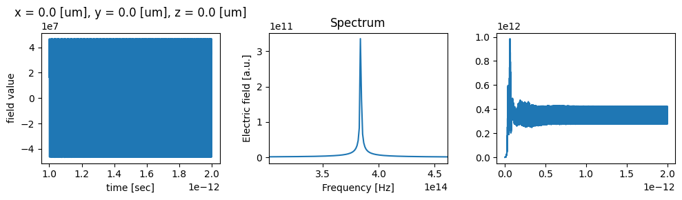
Now, we can visualize the SHG fields from the resonant mode:

[28]:

# Get data from the TimeMonitor
tdata = sim_data_SH["time_series"]

time_series = tdata.Ez.squeeze()

# Get data from the TimeMonitor
tdata_flux = sim_data_SH["flux_time"]

flux = tdata_flux.flux.squeeze()
time_flux = tdata_flux.flux.coords["t"]

fig, (ax1, ax2, ax3) = plt.subplots(1, 3, figsize=(10, 3))

# Plot time dependence
time_series.plot(ax=ax1)

# Make frequency mesh and plot spectrum
dt = sim_data_SH.simulation.dt
fmesh = np.linspace(-1 / dt / 2, 1 / dt / 2, time_series.size)
spectrum = np.fft.fftshift(np.fft.fft(time_series))

ax2.plot(fmesh, np.abs(spectrum))
ax2.set_xlim(2 * freq0 - 2 * fwidth, 2 * freq0 + 2 * fwidth)
ax2.set_xlabel("Frequency [Hz]")
ax2.set_ylabel("Electric field [a.u.]")
ax2.set_title("Spectrum")

ax3.plot(time_flux, np.abs(flux))

plt.tight_layout()

plt.show()

[29]:

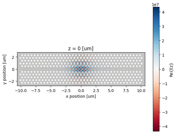
ax = sim_data_SH.plot_field("field_mnt", "Ez", "real", z=0, robust=False, eps_alpha=0, phase=np.pi)

ax.pcolormesh(eps.x, eps.y, eps.sel(z=0, method="nearest").real.T, alpha=0.2, cmap="binary")

plt.show()

Learning Center

Second harmonic generation¶

Parameters Definition¶

Gaussian Pulse Simulation¶

CW Run¶

Second Harmonic Simulation¶

More Notebooks