Author: Guodong Zhu, Vanderbilt University
In this instance, we replicate the absorption simulation as detailed by the work Sen Yang, Mingze He, Chuchuan Hong, Josh Nordlander, Jon-Paul Maria, Joshua D. Caldwell, and Justus C. Ndukaife, "Single-peak and narrow-band mid-infrared thermal emitters driven by mirror-coupled plasmonic quasi-BIC metasurfaces," Optica 11, 305-314 (2024) DOI:10.1364/OPTICA.514203. In this notebook, we emulate the same structure and demonstrate that our resultant absorption spectrum aligns closely with their published results.
import matplotlib.pylab as plt
import numpy as np
import tidy3d as td
import tidy3d.web as web
Simulation Setup
Define global variables
um = 1e0
nm = 1e-3
wavelength = 4 # central wavelength
freq = td.C_0 / wavelength # central frequency

# define frequency range
freq_high = td.C_0 / (wavelength - 1 * um)
freq_low = td.C_0 / (wavelength + 1 * um)
fwidth = freq_high - freq_low
spectrum_freq = np.linspace(freq - fwidth / 2, freq + fwidth / 2, 1000)
run_time = 200 / fwidth
Define materials.
medium_spacer = td.Medium(permittivity=1.685**2)
medium_gold = td.material_library["Au"]["Olmon2012evaporated"]
medium_substrate = td.Medium(permittivity=1.64**2)
eps_background = 1.0
Define geometric parameters used in the simulation.
thick_gold = 200 * nm
thick_sub = 4.2
thick_spacer = 0.65
thick_reflector = 0.15
thick_air = 4.8
Define the simulation domain size.
size_x = 2100 * nm
size_y = 2100 * nm
size_z = thick_sub + thick_gold + thick_air + thick_spacer + thick_reflector  # totsl 10 um
Calculate the center positions of the structures.
top_z = size_z / 2.0
center_air_z = top_z - thick_air / 2.0
center_metal_z = top_z - thick_air - thick_gold / 2.0
center_spacer_z = top_z - thick_air - thick_gold - thick_spacer / 2.0
center_reflector_z = top_z - thick_air - thick_gold - thick_spacer - thick_reflector / 2.0
center_sub_z = top_z - thick_air - thick_gold - thick_spacer - thick_reflector - thick_sub / 2.0
Create the structures.
from tidy3d import BoundarySpec, Boundary

reflector = td.Structure(
    geometry=td.Box.from_bounds(
        rmin=(-td.inf, -td.inf, center_reflector_z - thick_reflector / 2.0),
        rmax=(+td.inf, +td.inf, center_reflector_z + thick_reflector / 2.0),
    ),
    medium=medium_gold,
    name="reflector",
)

spacer = td.Structure(
    geometry=td.Box.from_bounds(
        rmin=(-td.inf, -td.inf, center_spacer_z - thick_spacer / 2.0),
        rmax=(+td.inf, +td.inf, center_spacer_z + thick_spacer / 2.0),
    ),
    medium=medium_spacer,
    name="spacer",
)

substrate = td.Structure(
    geometry=td.Box(
        center=(0, 0, -size_z + thick_sub),
        size=(td.inf, td.inf, size_z),
    ),
    medium=medium_substrate,
    name="substrate",
)

# (1) make a cylinder at origin
# (2) scale 0.21 in x, 0.7 in y
# (3) rotate 6 degree w.r.t z
# (4) move 0.525 um in +x direction
ellipse_R = td.Structure(
    geometry=td.Transformed(
        geometry=td.Cylinder(radius=1, center=[0, 0, 0.1], length=0.2),
        transform=[
            [0.20884959802733738, -0.07316992428735743, 0, 0.525],
            [0.021950977286207228, 0.6961653267577913, 0, 0],
            [0, 0, 1, 0],
            [0, 0, 0, 1],
        ],
    ),
    medium=medium_gold,
    name="ellipse_R",
)
# similar to right, move in -x direction and rotate -6 degree
ellipse_L = td.Structure(
    geometry=td.Transformed(
        geometry=td.Cylinder(radius=1, center=[0, 0, 0.1], length=0.2),
        transform=[
            [0.20884959802733738, 0.07316992428735743, 0, -0.525],
            [-0.021950977286207228, 0.6961653267577913, 0, 0],
            [0, 0, 1, 0],
            [0, 0, 0, 1],
        ],
    ),
    medium=medium_gold,
    name="ellipse_L",
)
Create a plane wave source as excitation. Create field monitors and flux monitors to record the field distribution and far-field reflection.
plane_wave = td.PlaneWave(
    center=(0, 0, center_air_z),
    size=(td.inf, td.inf, 0),
    source_time=td.GaussianPulse(freq0=freq, fwidth=fwidth),
    pol_angle=0,
    angle_theta=0,
    direction="-",
)

field_monitor_xy = td.FieldMonitor(
    center=(0, 0, center_metal_z),
    size=(td.inf, td.inf, 0),
    freqs=[freq],
    name="field_xy",
)

field_monitor_xz = td.FieldMonitor(
    center=(0, 0, 0),
    size=(td.inf, 0, td.inf),
    freqs=[freq],
    name="field_xz",
)

reflection = td.FluxMonitor(
    center=(0, 0, center_air_z + 1),
    size=(td.inf, td.inf, 0),
    freqs=spectrum_freq,
    name="reflection",
)
Add a mesh override structure to locally refine the grid around the structure for better accuracy.
mesh_overrides = [
    td.MeshOverrideStructure(
        geometry=td.Box.from_bounds(
            rmin=(-td.inf, -td.inf, center_reflector_z - thick_spacer / 2.0),
            rmax=(+td.inf, +td.inf, center_metal_z + thick_gold / 2.0),
        ),
        dl=[40 * nm, 40 * nm, 20 * nm],
    )
]
Create a simulation.
ellipse_TE = td.Simulation(
    size=(size_x, size_y, size_z),
    run_time=run_time,
    structures=[substrate, spacer, reflector, ellipse_R, ellipse_L],
    sources=[plane_wave],
    monitors=[field_monitor_xy, field_monitor_xz, reflection],
    # grid_spec=td.GridSpec.uniform(dl=dl),
    boundary_spec=td.BoundarySpec(
        x=Boundary.periodic(),
        y=Boundary.periodic(),
        z=td.Boundary(plus=td.PML(num_layers=64), minus=td.PML(num_layers=12)),
    ),
    grid_spec=td.GridSpec.auto(
        wavelength=wavelength,
        min_steps_per_wvl=20,
        override_structures=mesh_overrides,
    ),
)
ellipse_TE.plot_3d()
# shift the plot positions a little so the field monitors don't overlap plots
shift_plot = 0.01
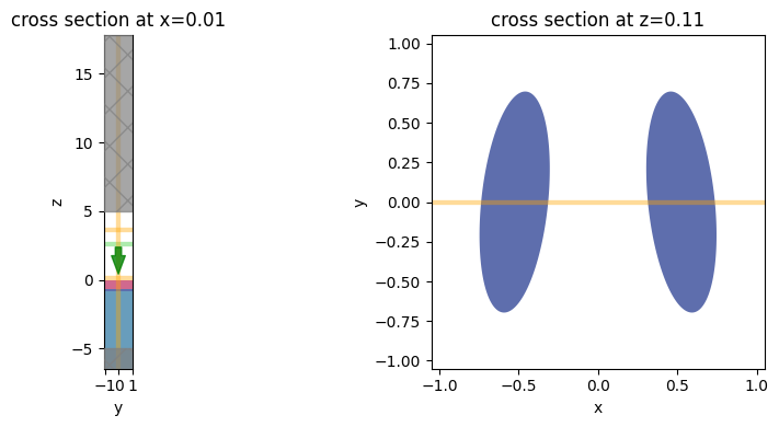
f, (ax1, ax2) = plt.subplots(1, 2, figsize=(10, 4), tight_layout=True)
ellipse_TE.plot(x=0.0 + shift_plot, ax=ax1)
ellipse_TE.plot(z=center_metal_z + shift_plot, ax=ax2)
plt.show()
Submit the Simulation and Visualize the Result
Now we run the simulation and plot the absorption spectrum first.
sim_data = web.run(ellipse_TE, task_name="thermal_emitter_ellipse", verbose=True)
16:45:23 UTC Created task 'thermal_emitter_ellipse' with task_id
             'fdve-d9e0e6c5-828e-4fb7-89fc-2270087c509a' and task_type 'FDTD'.
             View task using web UI at
             'https://tidy3d.simulation.cloud/workbench?taskId=fdve-d9e0e6c5-828
             e-4fb7-89fc-2270087c509a'.
Output()
16:45:24 UTC status = success
Output()
loading simulation from simulation_data.hdf5
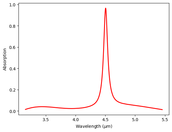
The absorption spectrum (1 - reflection) shows one narrow peak, indicating a high Q resonance. The result reproduces Fig.1 of the reference.
wavelengh = td.C_0 / spectrum_freq
reflection = sim_data["reflection"].flux
plt.plot(wavelengh, 1.0 - reflection, c='red', linewidth=2)
plt.xlabel("Wavelength ($\mu m$)")
plt.ylabel("Absorption")
plt.show()
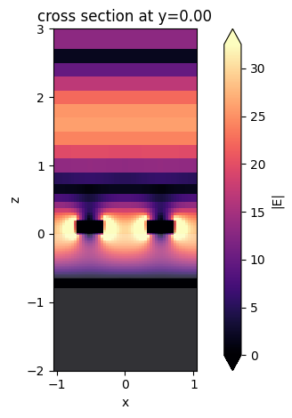
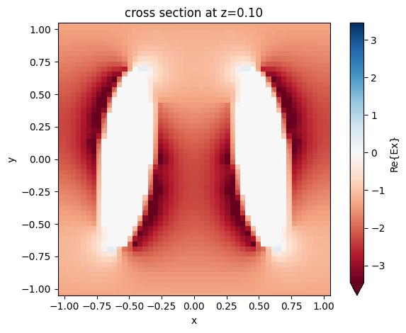
Finally we plot the field distributions from the field monitors.
sim_data.plot_field("field_xy", "Ex", "real")
plt.show()
ax = sim_data.plot_field("field_xz", "E", "abs")
ax.set_ylim(-2,3)
plt.show()