Author: Dr. Chenchen Wang, Postdoctoral Researcher at the University of Wisconsin–Madison.
In this notebook, we demonstrate the modeling of a waveguide-coupled nonlinear Kerr resonator using Tidy3D, followed by the generation of a Kerr frequency comb via continuous-wave pumping in the resonator. We employ monitors to display the intracavity spectral and temporal characteristics at different times during the early stages of Kerr comb formation. Our results are in good agreement with both theoretical predictions and experimental observations.
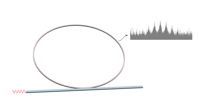
The model consists of a ring resonator coupled with a bus waveguide, fed with a ContinuousWave source. The resonator exhibits (\chi^{(3)}) nonlinearity and hence allows the formation of a Kerr comb over time. To observe the Kerr comb formation over time, we will add frequency-domain monitors with different apodization times to capture the spectral response at different time slots. We will also place a FluxTimeMonitor to observe the interference pattern forming over time due to the generation of Kerr sidebands.
This simulation includes around 11M grid points and 10M time steps, it will take approximately 50 credits and 1.5 hours to finish.
import numpy as np
import matplotlib.pyplot as plt

import tidy3d.web as web
import tidy3d as td
from tidy3d.plugins.mode import ModeSolver
Simulation Setup
# ---------------------------
# Parameter Definitions
# ---------------------------
# Geometrical parameters
wg_width = 1.25
couple_width = 0.5
ring_radius = 50
ring_wg_width = wg_width
wg_spacing = 2.5
buffer = 5.0

# Simulation dimensions
x_span = 2 * wg_spacing + 2 * ring_radius + 2 * buffer
y_span = 2 * ring_radius + ring_wg_width + wg_width + couple_width + 2 * buffer
sim_center_y = (couple_width + wg_width) / 2
wg_insert_x = ring_radius + wg_spacing
wg_center_y = ring_radius + ring_wg_width / 2.0 + couple_width + wg_width / 2.0

# Wavelength and frequency parameters
lambda_beg = 1.25
lambda_end = 2
f_middle = (td.C_0 / lambda_end + td.C_0 / lambda_beg) / 2
freq0 = 193.466e12  # Override calculated result
amp = 14
run_time = 750e-12
min_steps_per_wvl = 30

freq_beg = td.C_0 / lambda_end
freq_end = td.C_0 / lambda_beg
fwidth = (freq_end - freq_beg) / 2

# ---------------------------
# Medium Definitions
# ---------------------------
n_bg = 1.0
n_solid = 1.5
background = td.Medium(permittivity=n_bg**2)
solid = td.Medium(permittivity=n_solid**2)

n_kerr_2 = 2.0e-8
kerr_chi3 = 4 * (n_solid**2) * td.constants.EPSILON_0 * td.constants.C_0 * n_kerr_2 / 3
chi3_model = td.NonlinearSpec(
    models=[td.NonlinearSusceptibility(chi3=kerr_chi3)], num_iters=10
)
kerr_solid = td.Medium(permittivity=n_solid**2, nonlinear_spec=chi3_model)
# ---------------------------
# Structure and Simulation Region Definitions
# ---------------------------
# Define structure
waveguide = td.Structure(
    geometry=td.Box(
        center=[0, wg_center_y, 0],
        size=[td.inf, wg_width, td.inf],
    ),
    medium=solid,
    name="waveguide",
)
# Ring Structure
outer = td.Cylinder(
    center=[0, 0, 0],
    axis=2,
    radius=ring_radius + ring_wg_width / 2.0,
    length=td.inf,
)
inner = td.Cylinder(
    center=[0, 0, 0],
    axis=2,
    radius=ring_radius - ring_wg_width / 2.0,
    length=td.inf,
)
ring = td.Structure(
    geometry=outer - inner,
    medium=kerr_solid,
    name="outer_ring",
)
# Define mode plane and ring mode plane
mode_plane = td.Box(center=[-wg_insert_x, wg_center_y, 0], size=[0, 10, td.inf])
ring_mode_plane = td.Box(center=[0, -ring_radius, 0], size=[0, 10, td.inf])
# ---------------------------
# Mode Solver Setup
# ---------------------------
sim_modesolver = td.Simulation(
    center=[0, sim_center_y, 0],
    size=[x_span, y_span, 0],
    grid_spec=td.GridSpec.auto(
        min_steps_per_wvl=min_steps_per_wvl, wavelength=td.C_0 / freq0
    ),
    structures=[waveguide],
    run_time=1e-12,
    boundary_spec=td.BoundarySpec.all_sides(boundary=td.Periodic()),
    medium=background,
)

mode_spec = td.ModeSpec(num_modes=2)
mode_solver = ModeSolver(
    simulation=sim_modesolver, plane=mode_plane, mode_spec=mode_spec, freqs=[freq0]
)
mode_data = web.run(mode_solver, "mode_solver_kerr")
20:37:44 -03 Created task 'mode_solver_kerr' with task_id
             'mo-ce947ad7-a58c-46bd-b2d6-333c436ce22e' and task_type
             'MODE_SOLVER'.
             View task using web UI at
             'https://tidy3d.simulation.cloud/workbench?taskId=mo-ce947ad7-a58c-
             46bd-b2d6-333c436ce22e'.
Task folder: 'default'.
Output()
20:37:47 -03 Maximum FlexCredit cost: 0.004. Minimum cost depends on task
             execution details. Use 'web.real_cost(task_id)' to get the billed
             FlexCredit cost after a simulation run.
20:37:48 -03 status = success
Output()
20:37:50 -03 loading simulation from simulation_data.hdf5
f, ((ax1, ax2, ax3), (ax4, ax5, ax6)) = plt.subplots(
2, 3, tight_layout=True, figsize=(10, 6)
)
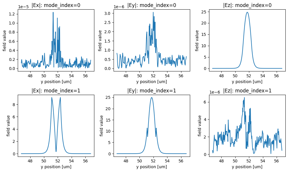
mode_data.Ex.sel(mode_index=0, f=freq0).abs.plot(ax=ax1)
mode_data.Ey.sel(mode_index=0, f=freq0).abs.plot(ax=ax2)
mode_data.Ez.sel(mode_index=0, f=freq0).abs.plot(ax=ax3)
mode_data.Ex.sel(mode_index=1, f=freq0).abs.plot(ax=ax4)
mode_data.Ey.sel(mode_index=1, f=freq0).abs.plot(ax=ax5)
mode_data.Ez.sel(mode_index=1, f=freq0).abs.plot(ax=ax6)
ax1.set_title("|Ex|: mode_index=0")
ax2.set_title("|Ey|: mode_index=0")
ax3.set_title("|Ez|: mode_index=0")
ax4.set_title("|Ex|: mode_index=1")
ax5.set_title("|Ey|: mode_index=1")
ax6.set_title("|Ez|: mode_index=1")
mode_data.to_dataframe()
| wavelength | n eff | k eff | TE (Ey) fraction | wg TE fraction | wg TM fraction | mode area | ||
|---|---|---|---|---|---|---|---|---|
| f | mode_index | |||||||
| 1.934660e+14 | 0 | 1.549587 | 1.429314 | 0.0 | 1.222074e-14 | 1.000000 | 0.931953 | 1.172565 |
| 1 | 1.549587 | 1.404287 | 0.0 | 1.000000e+00 | 0.881685 | 1.000000 | 1.304658 |
# ---------------------------
# Monitor Settings
# ---------------------------
# Define measurement frequency range for the ring mode monitors
lambdas_measure = np.linspace(lambda_beg, lambda_end, 1001)
freqs_measure = td.C_0 / lambdas_measure[::-1]
# Create multiple ring mode monitors with different time windows using a loop
pulses = [[40, 50], [400, 410], [600, 610], [730, 740]]
ring_mode_monitors = []
for i, pulse in enumerate(pulses, start=1):
apodization = td.ApodizationSpec(
start=1e-12 * pulse[0], end=1e-12 * pulse[1], width=2e-13
)
monitor = td.ModeMonitor(
size=ring_mode_plane.size,
center=ring_mode_plane.center,
freqs=freqs_measure,
mode_spec=td.ModeSpec(num_modes=2),
apodization=apodization,
name=f"ring_mode_{i}",
)
ring_mode_monitors.append(monitor)
# Define output flux monitor
out_flux_monitor = td.FluxTimeMonitor(
size=ring_mode_plane.size,
center=ring_mode_plane.center,
name="out_flux",
)
# ---------------------------
# Source Definition
# ---------------------------
mode_source = td.ModeSource(
size=mode_plane.size,
center=mode_plane.center,
source_time=td.ContinuousWave(freq0=freq0, fwidth=fwidth, amplitude=amp),
mode_spec=td.ModeSpec(num_modes=2),
mode_index=1,
direction="+",
num_freqs=11,
)
# ---------------------------
# Overall Simulation Setup
# ---------------------------
sim = td.Simulation(
normalize_index=None,
center=[0, sim_center_y, 0],
size=[x_span, y_span, 0],
grid_spec=td.GridSpec.auto(
min_steps_per_wvl=min_steps_per_wvl, wavelength=td.C_0 / f_middle
),
structures=[waveguide, ring],
sources=[mode_source],
monitors=[out_flux_monitor] + ring_mode_monitors,
run_time=run_time,
boundary_spec=td.BoundarySpec(
x=td.Boundary.pml(), y=td.Boundary.pml(), z=td.Boundary.periodic()
),
medium=background,
shutoff=0,
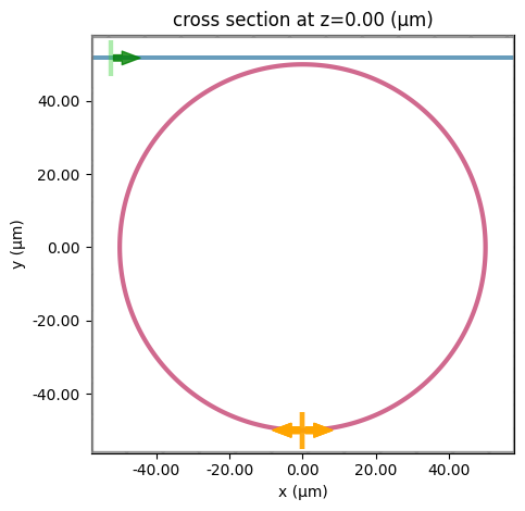
)
sim.plot(z=0)
plt.show()
20:37:51 -03 WARNING: The monitor 'interval' field was left as its default
             value, which will set it to 1 internally. A value of 1 means that
             the data will be sampled at every time step, which may potentially
             produce more data than desired, depending on the use case. To
             reduce data storage, one may downsample the data by setting
             'interval > 1' or by choosing alternative 'start' and 'stop' values
             for the time sampling. If you intended to use the highest
             resolution time sampling, you may suppress this warning by
             explicitly setting 'interval=1' in the monitor.
Running Simulation
# ---------------------------
# Run Simulation Task
# ---------------------------
sim_data = web.run(
    sim,
    task_name=f"2DKerrFC_{freq0*1e-12:.3f}1550_Runtime{run_time*1e12:.3f}_Amp{amp}",
    path="data/simulation_data.hdf5",
    verbose=True,
)
             WARNING: Simulation has 9.47e+06 time steps. The 'run_time' may be
             unnecessarily large, unless there are very long-lived resonances.
             Created task '2DKerrFC_193.4661550_Runtime750.000_Amp14' with
             task_id 'fdve-5f43a1d6-282b-4caf-b38c-cec7093eb9a1' and task_type
             'FDTD'.
             View task using web UI at
             'https://tidy3d.simulation.cloud/workbench?taskId=fdve-5f43a1d6-282
             b-4caf-b38c-cec7093eb9a1'.
Task folder: 'default'.
Output()
20:37:54 -03 Maximum FlexCredit cost: 46.632. Minimum cost depends on task
             execution details. Use 'web.real_cost(task_id)' to get the billed
             FlexCredit cost after a simulation run.
20:37:55 -03 status = success
Output()
20:38:11 -03 loading simulation from data/simulation_data.hdf5
             WARNING: Warning messages were found in the solver log. For more
             information, check 'SimulationData.log' or use
             'web.download_log(task_id)'.
We can see some warnings in the log due to non-decaying fields at the end of the simulation, which is the expected behavior when using ContinuousWave. Hence, the warning can be safely disregarded.
Analyzing Results
fig, axes = plt.subplots(nrows=4, ncols=1, figsize=(10, 15))
for i in range(4):
    # Extract amplitude data, convert to dB scale, and convert frequency to THz
    monitor = sim_data.monitor_data[f"ring_mode_{i+1}"]
    log_data = 20 * np.log10(
        np.array(monitor.amps.abs.sel(mode_index=1, direction="-"))
    )
    freqs = np.array(monitor.amps.f) / 1e12  # convert Hz to THz

    # Plot vertical lines representing the frequency spectrum
    axes[i].vlines(freqs, ymin=-320, ymax=log_data, color="gray")
    axes[i].set_ylim(-320, -200)
    axes[i].set_title(f"Frequency Spectrum at {sum(pulses[i]) / 2} ps")

    # Remove y-axis tick labels and add y-axis label
    axes[i].set_yticklabels([])
    axes[i].set_ylabel("Power 20 dB / div")

    # Label the x-axis with frequency in THz
    axes[i].set_xlabel("Frequency (THz)")

plt.tight_layout()
plt.show()
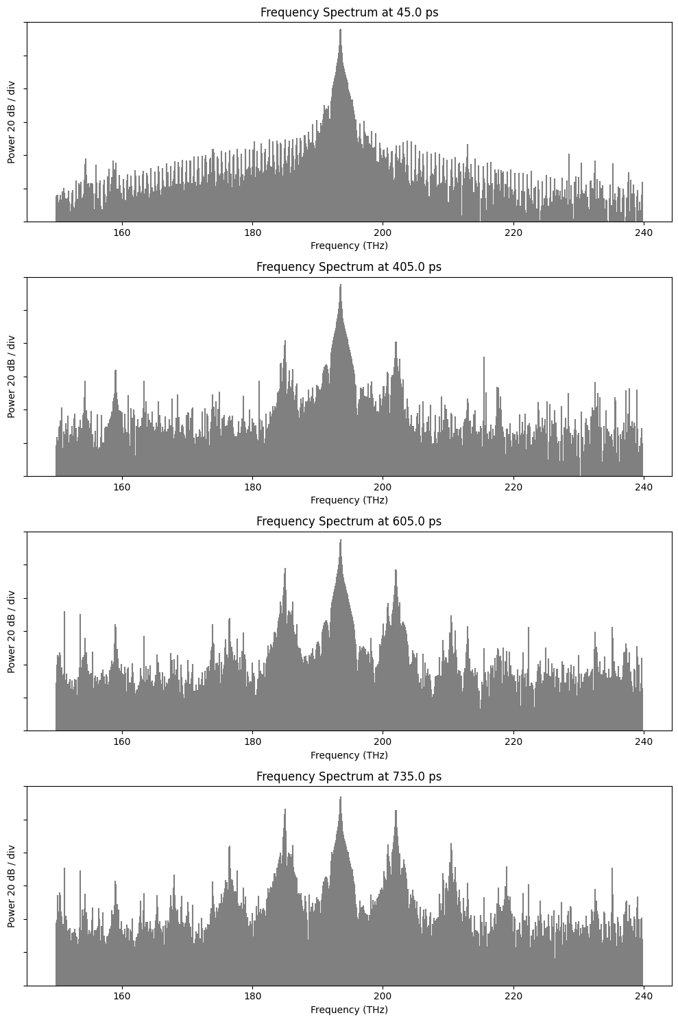
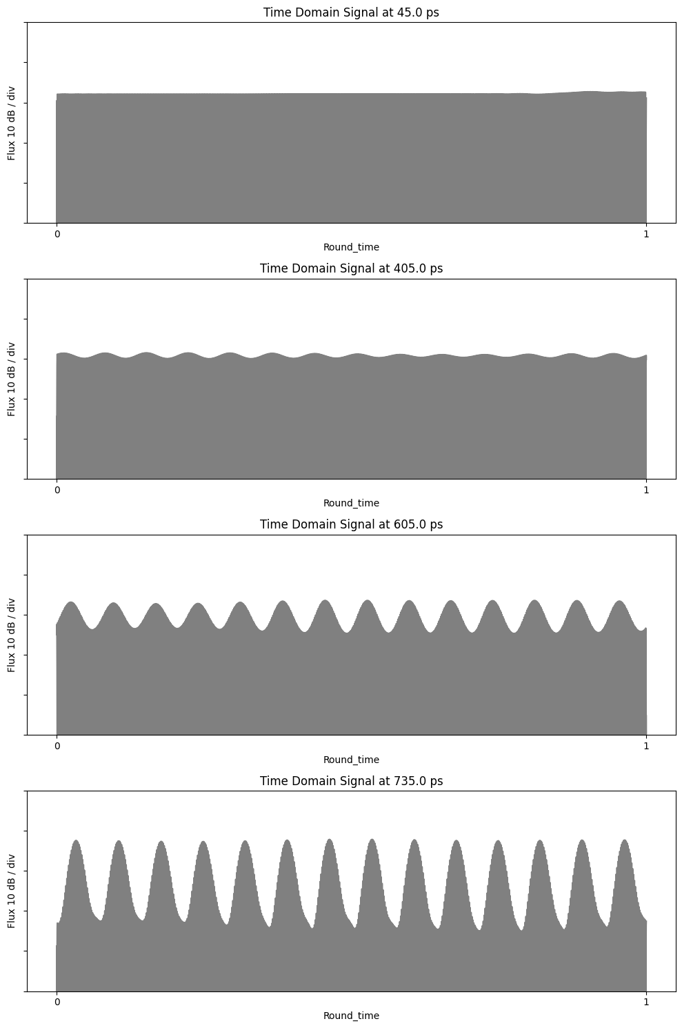
Now, we can plot the flux in the time domain over a round-trip time in the resonator for different time frames, showing the interference pattern forming due to Kerr comb frequency generation.
import os
import numpy as np
import matplotlib.pyplot as plt
from PIL import Image
from IPython.display import display, Image as IPyImage

# ---------------------------
# Measuring round time
# ---------------------------
Round_time = 1.643115e-12  # Duration per segment (s)

# ---------------------------
# Time Data Processing
# ---------------------------
time_data = np.abs(sim_data.monitor_data["out_flux"].flux)
time_data = np.log10(time_data)  # Convert to log scale)

total_duration = sim_data.simulation.run_time  # in seconds
total_samples = len(time_data)
dt = total_duration / total_samples
time_axis = np.linspace(0, total_duration, total_samples)  # in seconds
time_axis_ps = time_axis * 1e12  # convert to ps

# ---------------------------
# Animation Frame Generation with Time Annotation
# ---------------------------
frame_dir = "frames"
os.makedirs(frame_dir, exist_ok=True)

segment_samples = int(total_samples * (Round_time / total_duration))
segment_samples = max(segment_samples, 1)
num_frames = total_samples // segment_samples
print(
    f"Total samples: {total_samples}, Samples per frame: {segment_samples}, Total frames: {num_frames}"
)

frames = []
fig, ax = plt.subplots(figsize=(10, 4), dpi=100)
for i in range(num_frames):
    start_idx = i * segment_samples
    end_idx = start_idx + segment_samples
    if end_idx > total_samples:
        break  # Avoid out-of-bound indices
    segment = time_data[start_idx:end_idx]

    ax.clear()
    ax.plot(segment, color="gray")
    ax.set_ylim(2, 4.5)
    ax.set_xticks([])
    ax.set_yticks([])
    ax.set_frame_on(False)

    # Calculate current simulation time (in ps) for the frame and quantize to nearest 10 ps
    current_time = (i / (num_frames - 1)) * (run_time * 1e12)
    displayed_time = round(current_time / 10) * 10
    ax.text(
        0.05,
        0.9,
        f"Time: {displayed_time} ps",
        transform=ax.transAxes,
        color="black",
        fontsize=12,
    )

    fig.canvas.draw()
    image = np.array(fig.canvas.renderer.buffer_rgba())
    image_pil = Image.fromarray(image)
    frames.append(image_pil)

plt.close(fig)

gif_path = "time_series_animation.gif"
frames[0].save(gif_path, save_all=True, append_images=frames[1:], duration=100, loop=0)
print(f"GIF generated and saved as {gif_path}")
display(IPyImage(filename=gif_path))

# ---------------------------
# Time-Domain Plot with 4 Normalized Subplots
# ---------------------------
fig, axes = plt.subplots(nrows=4, ncols=1, figsize=(10, 15))
for i, pulse in enumerate(pulses):
    pulse_start_ps = (sum(pulse) - Round_time * 1e12) / 2
    pulse_end_ps = (sum(pulse) + Round_time * 1e12) / 2
    mask = (time_axis_ps >= pulse_start_ps) & (time_axis_ps <= pulse_end_ps)
    segment_time_ps = time_axis_ps[mask]
    segment_data = time_data[mask]

    # Normalize time: 0 at pulse_start and 1 at pulse_end
    normalized_time = (segment_time_ps - pulse_start_ps) / (
        pulse_end_ps - pulse_start_ps
    )

    axes[i].plot(normalized_time, segment_data, color="gray")
    axes[i].set_title(f"Time Domain Signal at {np.mean(pulse):.1f} ps")
    axes[i].set_ylim(2, 4.5)
    axes[i].set_xticks([0, 1])
    axes[i].set_xlabel("Round_time")
    axes[i].set_yticklabels([])
    axes[i].set_ylabel("Flux 10 dB / div")
plt.tight_layout()
plt.show()
/home/filipe/anaconda3/lib/python3.11/site-packages/xarray/core/computation.py:824: RuntimeWarning: divide by zero encountered in log10
  result_data = func(*input_data)
Total samples: 9472246, Samples per frame: 20751, Total frames: 456
GIF generated and saved as time_series_animation.gif
<IPython.core.display.Image object>